Estimating correlations between noisy activity patterns. A tricky problem with a generative solution.
In the quest to better understand brain function, we want to know how the complex patterns of neural activity, which can be observed using modern neuroimaging techniques (i.e., array recoding, fMRI, or M/EEG), relate to the tasks that the brain is engaged in. In this endeavour, we often want to know how similar two activity patterns are to each other. If two tasks (let's call them A and B) activate a specific brain region in a similar way, we can infer that this brain region does something similar in the two conditions. In this approach, we are not so much concerned with whether task A activates the region more than task B - rather we want to know how similar, or overlapping, brain activity patterns are - that is, we are interested in the correlation between the two activity patterns. Of course, sometimes we do care about the amount of activation, in which case correlations are not the right measure. But that's a different topic (Walther et al., 2016). The question of the correlation between two activations patterns comes up a lot. Does encoding and retrieval of the same item lead to similar activity patterns? To what degree do the activity patterns during planning and execution overlap (Ariani et al., 2020)? How much does a pattern related to a specific movement change with training (Berlot et al., 2020)? Estimating the true correlation between two patterns, however, can be extremely tricky.
So what's the problem?
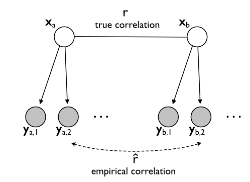
Statistically speaking, we are interested in the correlation between two vectors $\mathbf{x}_A$ and $\mathbf{x}_B$. Easy, you may say - just correlate the two vectors. But here is the hitch: we don't actually have the true activity patterns. Rather, we measure each of the patterns with noise - and if we use functional magnetic resonance imaging (fMRI), we have lot of it. Graphically, we can represent the situation as depicted in Figure 1. We are interested in the correlation between two true (but unobservable) activation patterns $\mathbf{x}_A$ and $\mathbf{x}_B$. We have a range of observations of each activity pattern $\mathbf{y}_{a,1}, \mathbf{y}_{a,2},...$ which differ from the true patterns by the measurement noise.
The obvious way to go about this, is to average the patterns across our repeated measurements for the two tasks, resulting in $\bar{\mathbf{y}}_a$ and $\bar{\mathbf{y}}_b$, and then just correlate those mean patterns. However, the problem is that the empirical correlation underestimates the true correlation substantially. This phenomenon can be seen in the simulation shown in Figure 2. The individual measured correlations (green dots) tend to be below the true correlation (dashed line). As the signal / noise ratio decreases, this bias becomes more severe. In the extreme, when we have no signal, the correlation goes down to zero.
This is not a problem if we just want to test the hypothesis that the true correlation is larger than zero. We can just calculate the individual correlations per subject and test them against zero using a t-test. However, sometimes we want to test whether the true correlation has a specific value (for example $r=1$, indicting that the activity patterns are the same), or we want to test whether the correlations are higher in one brain area than another. Different brain regions measured with fMRI often differ dramatically in their signal-to-noise ratio. Thus, in these cases we need to take into account our level of measurement noise.
Solution 1a: Compute noise ceilings
The first idea is to determine by how much our correlation estimate is biased. If we just knew this number, we should be able correct for it. To figure this out, we can ask ourselves what the correlation between two measured activity patterns would be, if the true activity patterns were perfectly correlated. This is often called the noise ceiling for the correlation.
To derive this quantity, we need to do a little bit of math. For simplicity let's assume that the two true patterns are identical ($\mathbf{x}_A$ = $\mathbf{x}_B$, and hence perfectly correlated). We further assume that the measure patterns consist of the true pattern and measurement noise
$$ \begin{align} \mathbf{y}_{a,i} = \mathbf{x}_{a} + \epsilon_{a,i}\\ \mathbf{y}_{b,i} = \mathbf{x}_{b} + \epsilon_{b,i} \end{align} $$
and that each of the terms has a specific variance (across voxels and repetitions).
$$ \begin{align} var(\mathbf{x}_a)=var(\mathbf{x}_b)=\sigma^2_{s}\\ var(\epsilon_a^2) = \sigma^2_{\epsilon a}\\ var(\epsilon_b^2) = \sigma^2_{\epsilon b} \end{align} $$
Then the correlation between two measures (assuming that their true patterns $\mathbf{x}_a$ and $\mathbf{x}_b$ are perfectly correlated), would be:
$$ \begin{align} r_{ceil}=\frac{cov(\mathbf{y}_{a},\mathbf{y}_b)}{\sqrt{var(\mathbf{y}_a)var(\mathbf{y}_b)}}=\frac{\sigma^2_s}{\sqrt{(\sigma^2_s+\sigma^2_{\epsilon a})(\sigma^2_s+\sigma^2_{\epsilon b})}} \end{align} $$
Now - how can we estimate the variance of the true pattern and the measurement noise? If we have multiple measures of our pattern, we can estimate the split-half reliability, the correlation between two independent halves of the data. If we assume that the noise has the same variance across these two halves, the expected value of the split-half correlation is:
$$ r_{rel,a}=r(\mathbf{y}_{a,1},\mathbf{y}_{a,2})=\frac{cov(\mathbf{y}_{a,1},\mathbf{y}_{a,2})}{\sqrt{var(\mathbf{y}_{a,1})var(\mathbf{y}_{a,2})}}=\frac{\sigma_s}{\sigma^2_s+\sigma^2_{\epsilon a}}. $$
By substitution in the previous formula, we can see that the noise ceiling for a correlation between two measured vectors (i.e., the value that we should get if the true vectors were perfectly correlated) is the geometric mean, the square-root of the product of their reliabilities. This is the noise ceiling for the correlation between A and B for two independent halves of the data. If we are interested in the noise ceiling for the correlation between the mean measured patterns, we need to extrapolate from the individual reliabilities ($r_i$) to the reliability of the mean across $N$ different measures ($r_m$), using the formula $r_m=r_i N /(r_i(N-1)+1)$.
$$ r_{ceil}=\sqrt{r_{rel,a} r_{rel,b}} $$
So now we should just be able to normalize our measured correlation by dividing it by the noise ceiling for correlation. As can be seen in Figure 3 (solid blue line) this works quite well if the signal to noise ratio is high. In this case the corrected estimate approaches the true correlation (black dashed line). For low signal-to-noise levels (and with fMRI we are usually in this domain) the correction stops working correctly. What is going on?
One problem is that in some cases $r_{rel,a}$ or $r_{rel,b}$ (or both) become negative, so that a real square root does not exist anymore. Here we have two options: Either we exclude these values from further analysis (blue solid line), or we replaced them with a specific value, for example $0$ (blue dashed line). Latter process is called imputation. Unfortunately, neither exclusion nor imputation fixes the problem. Both procedures show initially a positive bias, switching into a negative bias for very low signal to noise values. In general the problem is that the estimates become quite unstable when one of the reliabilities gets small.
Solution 1b: Use cross-partition covariances
A related solution is to use so-called "cross-validated" estimates of the correlation (Walther et al., 2016). Here, we calculate the correlation as usual, but estimate the variance and covariances of the patterns from the covariances across the $N$ different independent measures of the patterns (i.e., across blocks, or partitions). For the covariance estimator, we are only using estimates from different blocks. This makes sense for fMRI, as estimates for different task from a single imaging run are often correlated.
$$ \begin{align} \hat{cov}(\mathbf{x}_a,\mathbf{x}_b) = \frac{1}{N(N-1)}\sum_{i \neq j}cov(\mathbf{y}_{a,i},\mathbf{y}_{b,j})\\ \hat{var}(\mathbf{x}_a) = \frac{1}{N(N-1)}\sum_{i \neq j}cov(\mathbf{y}_{a,i},\mathbf{y}_{a,j}) \end{align} $$
We can then plug in these unbiased estimators into our correlation formula to obtain a cross-block (cb) estimator of the correlation:
$$ r_{cb}=\frac{\hat{cov}(\mathbf{x}_a,\mathbf{x}_b)}{\sqrt{\hat{var}(\mathbf{x}_a)\hat{var}(\mathbf{x}_a)}}. $$
This correlation (Figure 3, red line) behaves very similar to the noise-ceiling corrected estimator. Indeed, if you dig a bit through the math, you will realize that they differ only in one subtle way: solution 1a uses a ratio of correlations, whereas solution 1b uses a ratio of covariances instead. Again we have the problem that some of our variance estimator can become very small or negative, leading to the same issue of unstable or missing correlation estimates.
Solution 2: Using Pattern Component Modelling
Ok, so what can we do instead? Obtaining unbiased estimates of the true correlation, is, as we have seen, very tricky. The best solution therefore is to turn the problem around: Rather than asking which correlation is the best estimate given the data, let's instead ask how likely the data is given different levels of correlation. We can do this by using the generative model shown in Figure 1 combined with the assumption of normal distributions for the true patterns and noise. Then we can calculate $p(Y|r)$, the probability of the data given a specific correlation $r$. The technical details of model fitting and evaluation are implemented in the Pattern Component Modelling (PCM) toolbox (Diedrichsen et al., 2018), for which we have recently released a Python version.
Figure 4 shows an example of this approach. The light gray lines indicate the log-likelihood ($log p(Y|r)$) of individual data sets given true correlations between 0 and 1. Note that the actual value of the log-likelihood can vary widely with the scaling of the data. The only thing that can be interpreted are differences in the log-likelihood of the same data under different models. Here, we have therefore subtracted the mean log-likelihood across models from every curve. The gray dot on each line is the maximum-likelihood estimate of the true correlation, which we can obtain by fitting a model that has a free correlation parameter. While this estimate behaves a bit better than the noise-ceiling-corrected or cross-block estimates of the correlation, it still is not unbiased. For example, you could not test the hypothesis that the true correlation is 1. You would likely get a significant result even if the true correlation was 1, as the estimates can be smaller, but not larger than this value.
The rescue, however, is that we have the full likelihood curves for each participants. As you can see, some of these curves are quite flat - indicating that the data is nearly equally likely under all correlations. This is the case where the measured patterns were not very reliable and hence give us little information about the true correlation. Some of the likelihood curves have a clear peak - these are cases with reliable activity patterns which provide more information. The maximum of the mean log-likelihood curve (red solid line) is close to the true correlation of $0.7$.
One way to test specific hypothesis is to use standard frequentist tests with the differences in log-likelihood as the dependent variable. For example, does the correlation model of $0.7$ fit the data better than a model that assumes perfect correlation? When we conduct the paired t-test across the $20$ log-likelihood estimates, we find that $t(19)=0.029, p=0.97$ would not be significant. On the other hand, a correlation of $0.7$ would be significantly more likely than a correlation of $0.65$.
Instead of using frequentist test, we can also use the likelihoods in a Bayesian group analysis for a good introduction, see Stephan et al. (2009). If we assume that all correlations between $-1$ and $1$ are equally probable a priori, we can simply take the exponential of the log-likelihood and normalize the resulting probabilities to 1, giving us an approximate posterior distribution on the individual correlation. In this setting, a difference in log-likelihood of larger than $1$ is considered "worth talking about" (Kass & Raftery, 1995).
Extensions
The situation considered here with two activity patterns and two measures per activity pattern is quite simple. In most experiments, we have more complicated scenarios. Often want to know the correlation between patterns associated with specific items observed under two conditions. For example, we want to know how the patterns associated with 3 different movements correlate (on average) across observation and execution. In this scenarios we need integrate evidence across the 3 items, while also modelling the general differences between the 2 conditions (i.e., observation vs. execution). Additionally, we often need to account for the correlation between patterns in an imaging run, or different co-variance between the patterns for different items. Coming up with a good solution for all these problems using the noise-ceiling or cross-block approach can be quite difficult. I find it much easier to add these details into the generative model. An implementation of the above example can be found in the PCM toolbox documentation example.
Three take-homes
- Correlations estimated on noise data underestimate true correlations, making it difficult to test any hypothesis other than testing against zero.
- Correction of the correlations using a noise ceiling (or using cross-validated correlations) provides valid answers when the signal-to-noise is high. However, when the signal-to-noise level is low, as typical in fMRI analyses, these approaches become biased and unstable.
- Using the entire log-likelihood function across correlations of different sizes allows us to test specific hypothesis even if the signal-to-noise level is low.
While the generative approach provides stable inferences even for noisy data, it is, as you can see from the example in Figure 4, no magic bullet that suddenly gives you significant results where there was only noise before. For example, while we could see that the correlation was larger than $0.6$, we could not distinguish between correlations anywhere between $0.7 - 1.0$. However, the generative approach provides a valid (and in the likelihood sense optimal) evaluation of the real evidence that you have in your data about the true correlation between two activity patterns. We therefore find this approach to be a highly useful element in our analysis toolkit.
References
Diedrichsen et al. (2018). Pattern component modeling: A flexible approach for understanding the representational structure of brain activity patterns. NeuroImage.
Stephan et al. (2009). Bayesian model selection for group studies. Neuroimage.
Kass & Raftery (1995). Bayes Factors. Journal of the American Statistical Association.
Walther et al. (2016). Reliability of dissimilarity measures for multi-voxel pattern analysis. NeuroImage.
Ariani et al. (2020). Motor planning brings human primary somatosensory cortex into movement-specific preparatory states. bioRxiv.
Berlot et al. (2020). A critical re-evaluation of fMRI signatures of motor sequence learning. eLife.