How do I use the method?
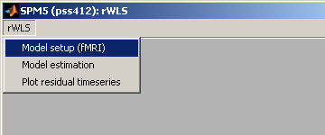
The toolbox provides modifications for two SPM-functions, Model setup (fMRI), and Estimation. Finally, it also has a function to visualize the residual time series (as in the example above).
 |
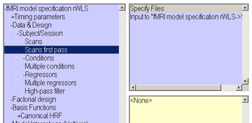
Model setup (fMRI)The basic functionality of this menu point is exactly the same as pressing the "fMRI" button in SPM. Indeed, specifying the design can be done using either the toolbox function or using the original function, with identical results. Thus, specify design, data, global normalization, and high-pass filtering as usual. |
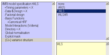 |
When specifying the covariance model, the new version gives two additional choices of auto-covariance models, 'WLS' and 'WLS_AR' additionally to the usual alternatives of 'none' and 'AR'. When choosing 'WLS', the algorithm will estimate the noise in each image on the first pass through the data, and then apply these estimates as weights in the second pass. When choosing 'WLS_AR', the algorithm will also attempt to simultaneously estimate the AR-coefficient to model temporal auto-correlation. |
 |
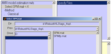
WLS works slightly better on unsmoothed data, so that it has enough independent data points to estimate the variance of the images. If rWLS does not converge on your smoothed and normalized data, you are given the option of whether the data for the first pass should be different from the main data. Enter here the unsmoothed data (however it should be realigned to correct for motion!) for the first pass, the estimation of variance-parameters. Two SPM-structures will be prepared and saved, the normal SPM.mat and an additional SPMfp.mat for the first pass. If you are using unsmoothed data anyway, just answer "no" and everything behaves as usual. |
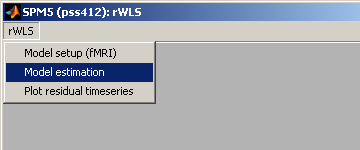 |
Model EstimationWhen
a model with and iid or AR co-variance model is specified (which can be setup with
the original SPM functions), this menu point does exactly the same as the
"Estimation" button in SPM (spm_spm.m). |
 |
If you specified the unsmoothed data for the first pass, choose SPMfp.mat when prompted for the SPM file. The program will estimate the noise parameters on the unsmoothed data and then automatically switch to SPM.mat to use the weights to analyze the smoothed data. |
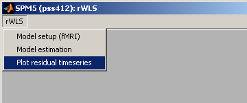 |
Plot residual time seriesThe new function provides some important diagnostic tools to see where in the time series the noise variance increased and whether WLS was successful in reducing it. Most of the information is stored in a new field in the SPM structure, SPM.resstats. This structure is the temporal equivalent to the residual mean-square image (see above). Noise-spikes from artifacts can so easily be detected and diagnosed. This structure is added even when no WLS model is chosen. |
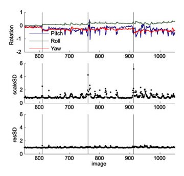 |
A number of statistics can be plotted:
Then you can specify which range (subset) of the images to be plotted. [1:300] only plots the the first 300 images. Enter [] for plotting all. Vertical lines indicate the start of each new scan (thin gray lines indicate events). |
Bugs / Fixes
24/10/2006: bug in spmj_all_onset fixed to deal with vertical onset vectors