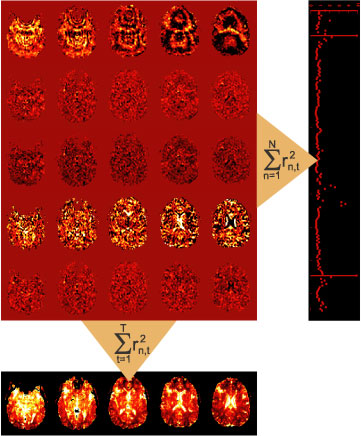The idea

The idea is simple: When we apply a linear model to imaging data, we are left with the residuals for each image (see images in red area). These residuals are only temporally saved in SPM. To summarize the residuals, they are squared and summed up over the whole timeseries. This results in the ResMS image (lower row) that reflects the variance estimate for each voxel. To detect artifacts, we propose to simply reverse the direction of summation: When adding up the squared residuals over the whole volume for each individual time point (right column), a residual-mean-square estimate for each image in the time-series will result.

This simple diagnostic can reveal images that are impacted by noise, for example noise caused by head motion. One function of the toolbox is to calculate this residual-mean-square time series during model estimation and to provide a diagnostic tool for plotting this together with the movement parameters. Thus, the toolbox can be used to do the classical estimation procedure (AR or iid model) and just adds a useful diagnostic tool.

When noise-artifacts are found in the data, the question arises of how to exclude those images. For example, images could be excluded based on an arbitrary threshold. We propose here use the statistically optimal approach: we can make use of the variance estimate for each image to weight each observation with the inverse of its variance. This leads to a "soft"-exclusion of images, the higher the variance of the image is, the less it will impact the results.

This approach has one problem: the residual-mean-square is not a unbiased estimate of the noise variance of each image. Rather, this measure is heavily influenced by the design matrix X. We therefore developed a Restricted Maximum Likelihood approach to obtain unbiased estimates of image variance, which then can be used weight the observations. Details on this approach can be found in Diedrichsen & Shadmehr (2005).

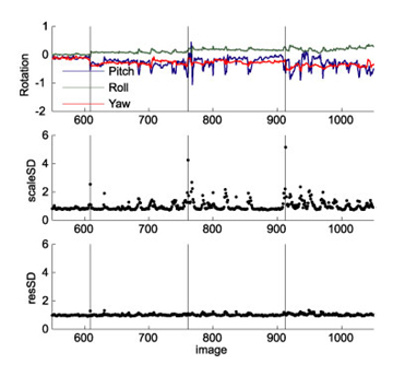Here a real example. It stems from a study with arm movements, using a bite bar for head stabilization. The particular participant started loosening his bite around TR 680, and consequently rotated his head slightly with every single arm movement. We used the rWLS approach to analyze the data.

In the first pass the algorithm estimated the noise variance of each image. Images that were taken while the head rotated showed an increase in noise variance by up to factor 9 (note that the SD of the images is plotted). The first image of each scan (black lines) also showed strongly increase noise variance.

Instead of excluding "bad" images, rWLS uses the factor 1/variance to weight the images in the second pass through the data. The last graph shows the mean squared residual for each image, after the weighting has been applied. Now the residual time series is homogenous, and we have obtained optimal model estimates from our (unfortunately) noisy data.