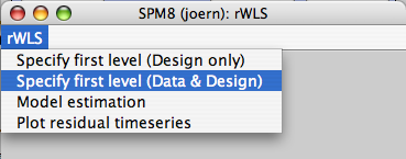
How do I use the method?
The toolbox provides modifications for the core SPM-functions for Model specification (Design only or Design & Data) and Estimation. It also has a function to visualize the residual time series. The new functions do not override any of the original functionality of SPM, but are accessible through the toolbox menu (toolbox->rwls) .
 |
Model setup (fMRI)The basic functionality of this menu point is exactly the same as the "specify 1st level" option in SPM. Indeed, specifying the design can be done using either the toolbox function or using the original function, with identical results. Specify design, data, global normalization, and high-pass filtering as usual. |
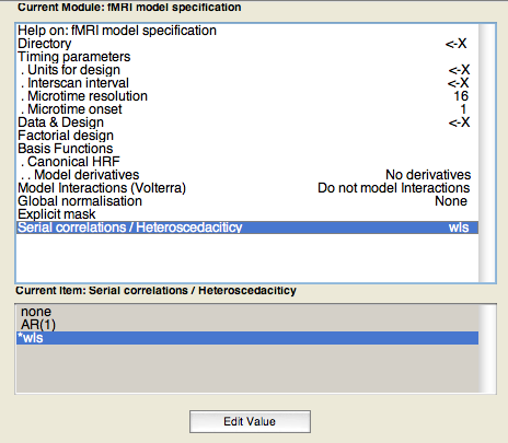 |
The only difference is the choice of covariance model (Serial correlations / Heteroscedasticity). The toolbox allows a new choice, 'WLS' additionally to the usual alternatives of 'none' and 'AR'. When choosing 'WLS', the algorithm will estimate the noise in each image on the first pass through the data, and then apply these estimates as weights in the second pass. Note that WLS works slightly better on unsmoothed data, so that it has more independent data points to estimate the variance of the images. We recommend not to smooth the raw data, but instead to smooth the beta-weights before submitting them to the second-level analysis. |
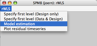 |
Model EstimationWhen
a model with an iid or AR co-variance model is specified (which can be setup with
the original SPM functions), this menu point does exactly the same as the
"Estimation" button in SPM (spm_spm.m). However, it adds the field
ResStats to the SPM structure to allow diagnostic of noisy images. |
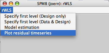 |
Plot residual time seriesThe plot function provides a diagnostic tools to see where in the time series the noise variance increased and whether WLS was successful in reducing it. The information is stored in a new field in the SPM structure, SPM.resstats. This structure is the temporal equivalent to the residual mean-square image (see above). Noise-spikes from artifacts can so easily be detected and diagnosed. This structure is added even when no WLS model is chosen. |
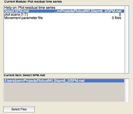 |
The first choice is the SPM-structure to be plotted. It need to be estimated with the estimation function from the toolbox. Secondly, you can specify which range (subset) of the images to be plotted. [1:300] only plots the noise parameters for the first 300 images. Leave this choice empty [] for plotting all. Vertical lines indicate the start of each new run. The last choice is the movement parameter file rp_*.txt. If this choice is left empty, the function will attempt to find this file automatically from the name of the first image of the first run. |
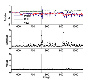 |
The translation and rotation parameters are shown in the first two panels. This allows you to determine if the artifacts are movement-related, or how much the realignment process was successful in canceling the movement. The third panel shows the estimates of the relative noise standard deviation before down-weighting of noisy scans. Here you should be able to see noise spikes and movement artifacts. This panel is only shown if the covariance structure of the model was specified as wls. The last panel gives the Residual mean square error as a function of scan, possibly after downweighting. If you used WLS, the noise spikes should have disappeared or at least be strongly attenuated. If you used the option "none" or "ar" the graph will show you how much the assumption of equal noise variance across images is violated. |