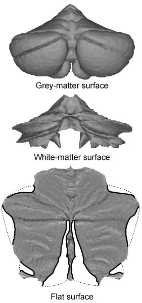
As part of the SUIT toolbox, we have developed a flat representation of the human cerebellum that can be used to visualise imaging data after volume-based normalisation and averaging across subjects. The method uses an approximate outer (grey-matter) and inner (white-matter) surface defined on the SUIT template (see figure to the left). Functional data between these two surfaces is projected to the surface along the lines connecting corresponding vertices. By applying cuts (thick black lines) the surface could be flattened out (bottom). We aimed to retain a roughly proportional relationship between the surface area of the 2D-representation and the volume of the underlying cerebellar grey matter. The map allows users to visualise the activation state of the complete cerebellar grey matter in one concise view, equally revealing both the anterior-posterior (lobular) and medial-lateral organisation. To explore the flatmap in more detail, check out our online cerebellar atlas viewer .
The surface representation of the cerebellum is a group surface, designed to display functional data that has been averaged across participants in volumetric group space. It does not rely on reconstructions of individual surfaces. While latter is the best practice for the neocortex, unfolding the cerebellar surface of individual subjects is very hard and requires anatomical scans of very high resolution and quality.
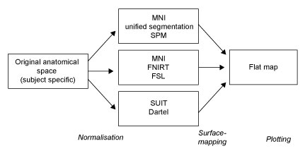
Thus there are three steps involved:
- Normalise data to a group space
- Map the data to the surface
- Display the data
For more details, see:
-
Diedrichsen, J. & Zotow, E. (2015). Surface-based display of volume-averaged
cerebellar data. PLoS One, 7, e0133402.

Surface mapping and display is implemented both in the Python and Matlab version of SUIT. Below follow instruction for the Matlab version.
Mapping
The functional data is typically normalised to the SUIT template, or to a MNI template
(using SPM's unified normalisation and segmentation routine, or FSL's nonlinear normalisation toolbox, FNIRT).
Although the three methods are rather close, they differ nonetheless in some details. To account for this
we have generated outer and inner surfaces for each of the three atlas spaces. It is therefore important to tell the mapping routine which method has been used to normalise the data.
The mapping uses both outer and inner surface. The vertices on the two surfaces come in pairs.
When mapping, the algorithm samples the image along the line connecting the two vertices and then takes the
mean of these numbers to determine the value of the vertex. When the underlying volume contains labels,
then the routine should take the mode. Finally, for statistical t-values, sometimes a glass-brain projection, using either the minimum or maximum, is desired. The mapping is achieve using the routine:
Data = suit_map2surf(image,'argument1',value1,'argument2',value2,...);
With the optional input arguments :
'space',{'SUIT/FSL/SPM'} |
Normalisation routine that was used for the group-normalisation of the data, determines the surface for sampling |
'depths',vec |
Depths at which the line is sampled. 0 refers to the outer surface, 1 to the inner surface. Default are 6 equally spaced positions along the line: [0 0.2 0.4 0.6 0.8 1] |
'stats', @fcn |
|
One can also save the mapped data in Gifti-format for display in surface-based imaging programs, such as the Connectome Workbench:
 C.cdata=suit_map2surf('myFile.nii');

C=gifti(C);

save(C,'mygiftifile.func.gii');
This can be useful, as the Connectome Workbench has a number of display options that are not easily achieved in Matlab.
Finally, the mapping routine can also map the location of activation foci (specified in terms of x,y,z in atlas space) to the flatmap. For this, simple pass a N x 3 matrix to the function, were every row is a seperate foci:
Foci=[22 -56 -28;12 -64 -46;30 -66 -56;6 -64 -10];

    Data=suit_map2surf(Foci,'space','SPM','depth_tolerance',3);
The first two columns of Data are the x and y positions of the foci on the flatmap. The last column indicates where between the pial and white surface the foci fell, with 0 corresponding to the pial and 1 to the white surface. If the coordinates do not fall between the two surfaces, NaN is returned for all values. The tolerance can be set with the optional input parameter 'depth_tolerance', which determines how many mm a foci can be above the pial or below the white surface to still be mapped on the surface. The foci can be then added as symbols to a flatmap, using a simple Matlab 'plot' command (for an example, see below).
Plotting
The map can then be plotted using the command
suit_plotflatmap(Data,'argument1',value1,'argument2',value2,...);
Data can be a 28935x1 vector, which correspond to the value of each vertex of the flatmap.If the type is set to 'rgb', the function expects a 28935x3 matrix, with r(ed), b(lue), and g(reen) values for each node. For places where the vector is NaN, the grey underlay will shine through. You have the option of also displaying the lobular boundaries (or other borders) as black dotted lines on the map.
Optional arguments are:
'underlay',file |
Specific a shape.gii file that dictates the shape of the grey underlay |
'underscale',[min max] |
Color scale to determine the value to color mapping for the underlay |
'undermap',Map |
Color map for the underlay, a N x 3 Matrix specifying RGB values [0..1] |
'type',type |
Data type to be shown, either |
'cmap',MAP |
Color map for the underlay, a N x 3 Matrix specifying RGB values [0..1] |
'cscale',[min max] |
Color scale: determines the mapping of values to color map |
'threshold',val |
show only values above this threshold |
'border',borderfile |
Specifies a borderfile to plot. Use [ ] for no borders. |
'bordersize',pt |
Weight of border points (default 8) |
'xlims',[xmin xmax] |
Limits of the x-coordinate |
'ylims',[ymin ymax] |
Limits of the y-coordinate |
'alpha',val |
Opacity of the overlay |
Examples
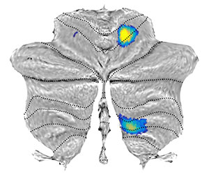 |
Map of representation of individual fingers of the right hand from Wiestler et al. (2011). The functional values are the z-value of the classification accuracy, with which the moved finger can be determined. The map clearly shows the anterior (Lobules V / VI) and posterior (Lobules VIII) hand region. The data ('ss1_motor_z.img') was normalised into SUIT space. The statistical function for the mapping is the mean across the voxel values for each vertices. For plotting we set the threshold to 1 and the color scale between 1 and 2. The default color-map is hot.
|
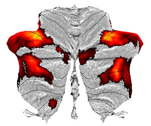 |
Plot t-values from a functional study in a glass-brain projection. The t-map indicates the load effect in a working memory task - it is the contrast between N-2 and N-0 back condition, which is part of the task-related studies of the Human Connectome project (Barch et al., 2013). The data was originally normalised using FSL's nonlinear MNI template (in which case the space would be 'FSL'). However, we have morphed the contrasts into SUIT space. In mapping we use the minmax function, which maps minimal or maximal values, so that all significant clusters can be see. For the flatmap display we are then using the colormap hot. cd SPM_HOME/toolbox/suit/functional_examples; |
 |
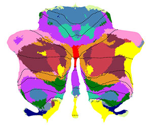
Plot the probabilistic lobular atlas (Diedrichsen et al., 2011) using the color map provided in the gifti file's label structure. Then it plots it without using borders. Load the gifti file |
 |
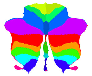
Map the labels of the resting state networks that indicate cerebellar-cortical connectivity (Buckner et al., 2011) onto a flat map. Here, we need to use the function mode to map the most-often occurring value. The data was transformed into SUIT space.
For plotting we then specify a colormap as a text file. The data is also available with a color map in the file |
 |
Map coordinates of previous studies onto the flat map. Here we chose the four peaks of in the meta-analysis for right hand motor task from Stoodley & Schmahmann (2009, Table 3). First we define the foci in x,y,z coordinates, with one row per foci: |
Details and acknowledgments:
The flatmap and software is made freely available as part of the SUIT toolbox. Please ensure that you acknowledge the following citation when using the map:
-
Diedrichsen, J. & Zotow, E. (2015). Surface-based display of volume-averaged
cerebellar data. PLoS One, 7, e0133402.